

Research
LEAP-HI: Compounding Risk and Mitigation Options for Building Infrastructure Experiencing Coastal Flooding-Related Saltwater Deterioration and Seismic Hazard
The selection of simulation events for model calibration and validation focused on those that generated high wave heights and water levels in the study area of Hilo, Hawaii. We selected two nearly simultaneous hurricane events: Hurricane Madeline (August 26, 2016, to September 03, 2016) and Hurricane Lester (August 24, 2016, to September 08, 2016) as they exhibited the largest half-hour significant wave height (5.37 m), and a relatively high hourly water level (0.664 m), recorded by the buoy and tide gauge stations, respectively, during the 2012-2023 period. The tracks of these two hurricane events are demonstrated in Figure 1, which shows that Hurricane Lester passed north of Hilo, while Hurricane Madeline passed south of Hilo.
Shoreline
Shoreline position is an essential input for the CMS model setup. Reliable and accurate shoreline data can assist in designing and building the model grid system. In this project, we adopted the National Oceanic and Atmospheric Administration (NOAA) Historical Composite Shoreline data as the shoreline input for the CMS modeling. This high-resolution vector shoreline data is based on a multi-temporal collection of NOAA shoreline T-sheets [5]. The average accuracy of the measured benchmarks is 3.06 m. Figure 2 shows the position of the shoreline within the study area.
Digital Elevation Model
Accurate and reliable topographic and bathymetric data are pivotal for CMS models. In this project, we adopted Digital Elevation Models (DEMs), which are cell-based digital surfaces representing the terrain, from three sources: (1) the 2013 USACE NCMP Topobathy Lidar (LMSL): Big Island, HI; (2) NOAA NCEI Continuously Updated Digital Elevation Model (CUDEM) – Ninth arc-second resolution bathymetric-topographic tiles: Hawaii; and (3) NOAA NCEI Continuously Updated Digital Elevation Model (CUDEM) – Third arc-second resolution bathymetric-topographic tiles: Hawaii [6–8]. The 2013 USACE NCMP Topobathy Lidar data were processed to create a DEM with a resolution of 1 m. The CUDEM datasets provide the nearshore topo-bathymetric DEM at a resolution of 1/9th arc-second (~3 m) and the offshore bathymetric DEM at a resolution of 1/3rd arc-second (~ 10 m). Figure 2 shows the combined DEM used in the coupled CMS model.
Manning’s n Value
Friction due to bottom roughness affects wave flow velocity. In this project, Manning’s roughness coefficient (n) is used to specify the bed roughness for the hydrodynamic calculations. Based on [9], two regions with different Manning’s n coefficients (0.075 and 0.085) are used in the model, as shown in Figure 3.
Water Level Data
In CMS, water level boundaries play a critical role in defining the exchange of water between the model domain and the surrounding environment. The general formula for the boundary water surface elevation (WSE) is:
where represents the boundary WSE (m), represents the initial boundary WSE (m), represents the specified external boundary WSE (m), Δη represents the WSE offset (m), represents the WSE component derived from user-specified gradients (m), represents the correction to the boundary WSE based on the wind and wave forcing (m), and represents the ramp function [10]. The external boundary WSE can be specified as a time series or calculated from tidal or harmonic constituents. In this project, we selected the water level time series from the tide gauge station NOAA 1617433, as shown in Figure 4, as the source for the external boundary WSE. This station (20.0367° N, 15.83° W), located at the Kawaihae Harbor Pier on the northern coast of the island of Hawaii, has collected water level data since 1988. Figure 5 shows the hourly water level data recorded in this station from August 29, 2016, to September 05, 2016.
Wave Data
The CMS-Wave model simulates spectral wave propagation over complex bathymetry and in nearshore environments, accounting for refraction, diffraction, reflection, shoaling, and breaking [10]. It requires directional spectral wave data as boundary input. In this project, we used the wave spectral data from the Wave Information Study (WIS) station ST83432 (19.8333° N, 154.8333° W), as shown in Figure 4. The WIS station provides a long-term (40+ years) hindcast of wave conditions generated using high-resolution wind fields, mean daily ice concentration fields, and the latest wave modeling technology [11]. The wave spectra data includes 35 directional bins with a 5-degree directional resolution and 29 frequency bins with frequencies ranging from 0.035 to 0.5047 Hz. The wave characteristics, including significant wave height, mean wave direction (the direction from which the waves travel), and wave period, for this station from August 29 to September 05, 2016, are shown in Figure 6.
Wind Data
Wind forcing is a critical input for CMS simulations because it directly drives the processes that generate and shape waves and has a significant impact on the accuracy and reliability of the model predictions. In this project, we obtained wind data from the WIS station ST83432, as shown in Figure 4. Figure 7 presents the wind speed (m/s) and wind direction (degrees). The wind direction indicates the direction from which the wind blows.
Model Setup and Parameters
In this project, two computational grids, i.e., the Quadtree grid for CMS-Flow and the Cartesian grid for CMS-Wave, were generated for the simulation. Figures 8 and 9 show the domain and spatial configuration of these two grids, respectively. The CMS-Flow Quadtree grid consists of 135,666 cells, with cell sizes ranging from 10 m near the breakwater to 320 m in the offshore region. The CMS-Wave Cartesian grid contains 382,130 cells (515 rows ×742 columns), and the cell sizes also range from 10 m near the breakwater to 320 m in the offshore region. The model control parameters for the CMS-Flow and CMS-Wave models are listed in Tables 1 and 2, respectively.
Results and Discussion
To evaluate the performance of the CMS model, simulated results were directly compared to observed data. The simulated water levels were compared to the data from the NOAA tide gauge station 1617760, located within Hilo Harbor, Hawaii. Figure 10 shows the comparison of simulated and measured water levels from August 29 to September 05, 2016. It shows that the simulated water levels aligned well with the observed water levels, though it slightly underestimated the peak and trough values. The root mean square error (RMSE) was 0.12 m, and the correlation coefficient was 0.86, as shown in Table 3. This indicates that the model has the capability to reproduce primary tidal dynamics.
The simulated significant wave heights were compared with the observations from the buoy station NDBC 51206 for the period from August 29 to September 05, 2016, as shown in Figure 11(a). The comparison shows that the timing of wave height peaks matched well, although the CMS model underestimated the magnitudes of the two peaks. This discrepancy may be attributed to the use of hindcast wave spectral data as the input, which may not fully capture extreme events. The RMSE of significant wave height was 0.51 m, and the correlation coefficient was 0.83, as shown in Table 3. Figure 11(b) presents the comparison of wave periods. It shows that the simulated results captured the overall pattern and temporal progression well. The RMSE was 1.26 seconds, and the correlation coefficient was 0.76, as shown in Table 3.
In summary, the results demonstrate that the coupled CMS-Wave and CMS-Flow models reliably simulate key coastal processes. Simulated water levels, significant wave heights, and wave periods showed consistently high correlation coefficients, and the RMSE values were within acceptable ranges. Discrepancies in wave height magnitudes and tidal extremes are likely due to limitations in the hindcast wave spectral input. Despite these limitations, the models effectively captured the temporal dynamics of the event and are suitable for flood inundation studies in Hilo, Hawaii.
By: Linqiang Yang, Oceana Francis University of Hawaii at Manoa. Last updated: July 15, 2025
Calibration and Validation of the Coastal Modeling System for Hilo, Hawaii


Figure 8. Model setup. Quadtree grid for the CMS-Flow model in the study area of Hilo, Hawaii
Table 1. Model setup. CMS-Flow model control parameters.
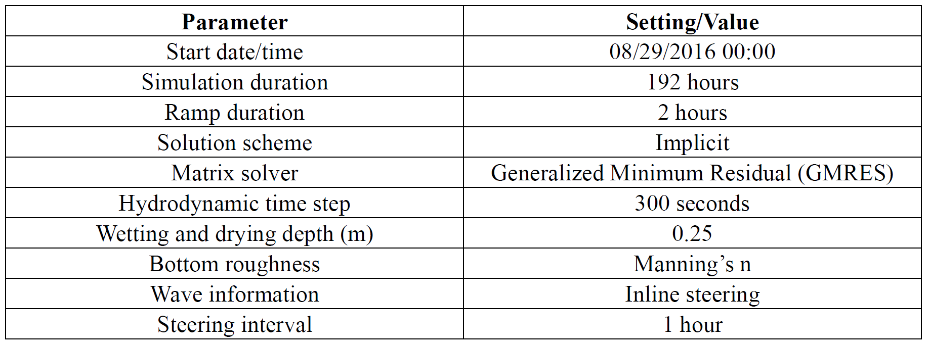

Figure 10. Results. Comparison of simulated (CMS) and observed (NOAA 1617760) water levels from August 29 to September 05, 2016.
Table 3. Results. Statistical comparison between observed and simulated water level, significant wave height, and wave period.
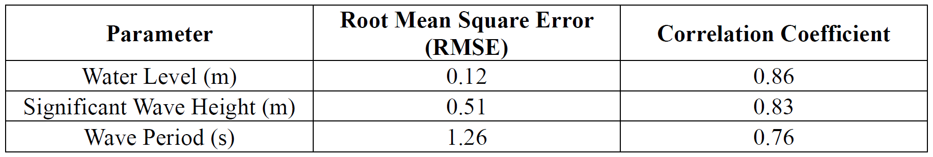


Figure 9. Model setup. Cartesian grid for the CMS-Wave model in the study area of Hilo, Hawaii.
Table 2. Model setup. CMS-Wave model control parameters.
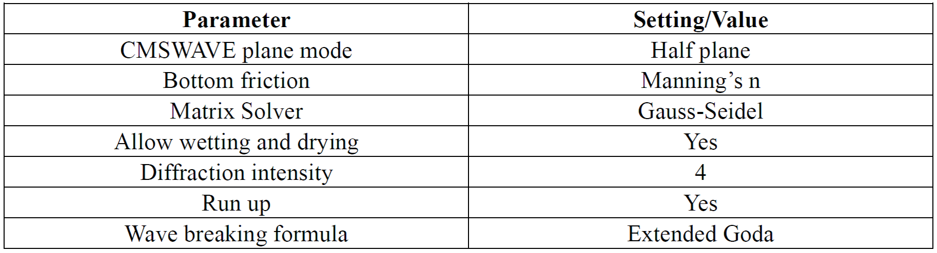
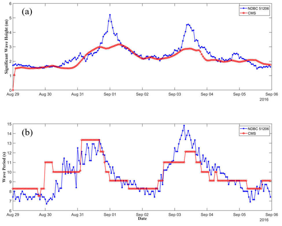
Figure 11. Results. Comparison of simulated (CMS) and observed (NDBC 51206) significant wave height (a) and wave period (b) from August 29 to September 05, 2016


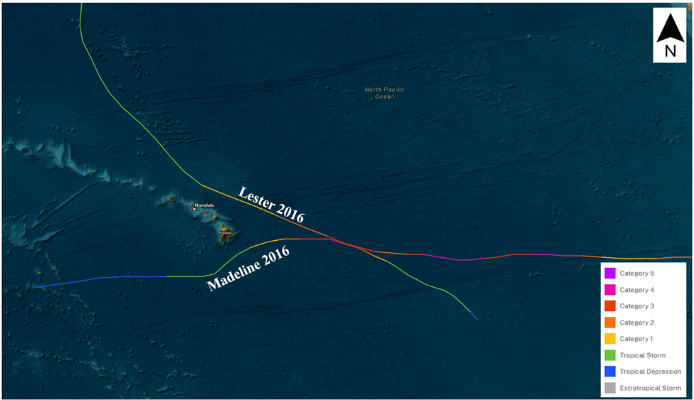
Figure 1. Tracks of Hurricane Madeline and Hurricane Lester on August 29, 2016 moving west towards Hilo (NASA, 2016)
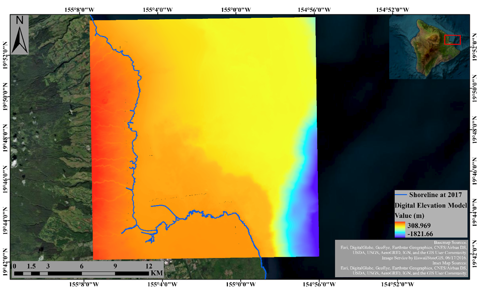
Figure 2. Digital Elevation Model (DEM) and shoreline position in the study area of Hilo, Hawaii.

Figure 3. Manning’s n values for bed roughness applied in the CMS model.
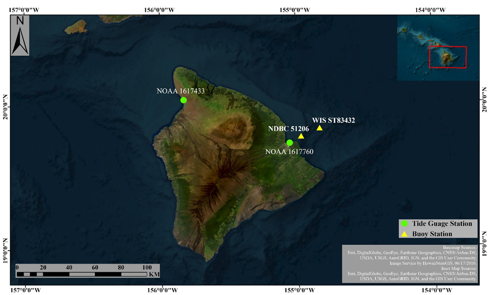
Figure 4. Locations of the tide gauge and buoy stations around Hawaii Island.
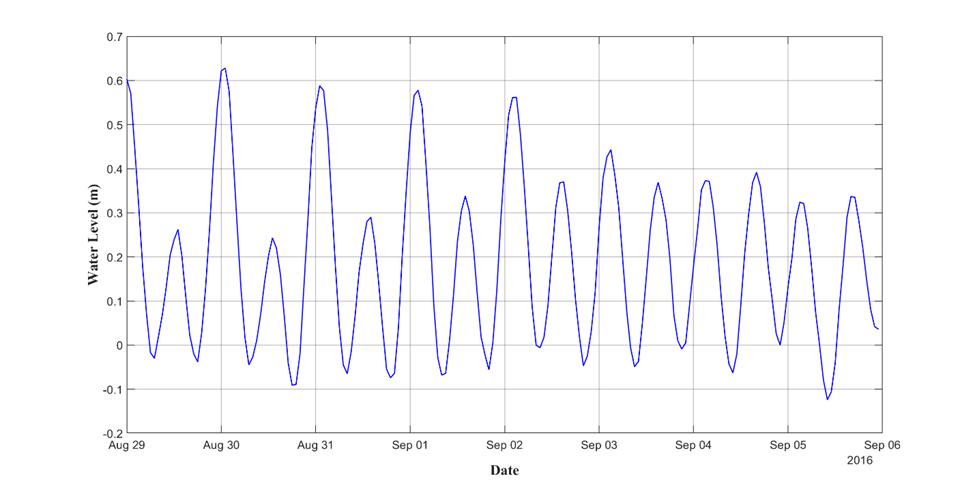
Figure 5. Hourly water level data at NOAA tide gauge station 1617433 from August 29 to September 05, 2016.
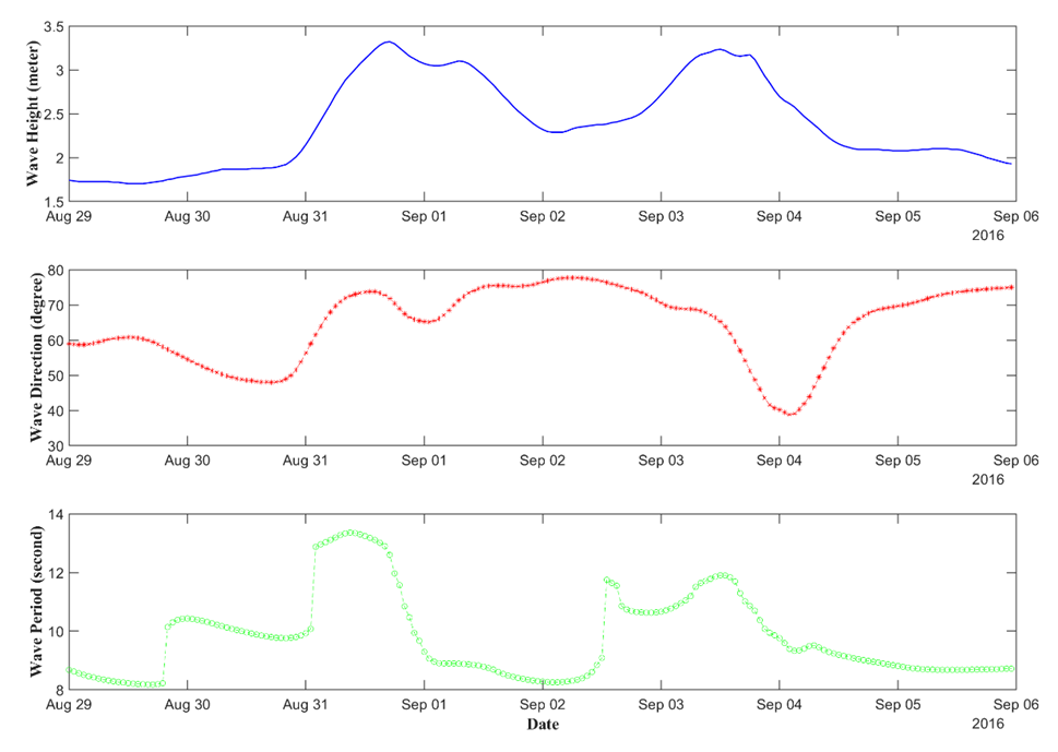
Figure 6. Wave characteristics for WIS station ST83432 from August 29 to September 05, 2016. Wave direction is the mean wave direction from which the waves are travelling.
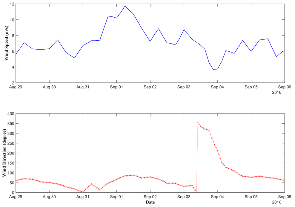
Figure 7. Wind data for WIS station ST83432 from August 29 to September 05, 2016. Wind direction is the direction from which the wind is blowing.